Lab 3: Acquiring and Analyzing Simulation Data

Author

John Murphy and Steven Carlson

Published

November 11, 2025

Learning Objectives

In this lab, you will bridge the gap between simulation and analysis. You will modify the C++ source code of a Geant4 application to save data and then use Python to analyze and visualize that data. By the end of this session, you will be able to:

Understand the basic structure of Geant4 user action classes
Modify C++ code to implement the G4AnalysisManager for data output
Save simulation results to CSV file format for universal compatibility
Write Python scripts using the pandas and matplotlib libraries
Load simulation data into pandas DataFrames
Create and customize histograms to visualize distributions
Calculate descriptive statistics (mean, standard deviation, percentiles) from data
Filter and manipulate data using pandas operations
Compare multiple datasets and create multi-plot figures

Introduction

A simulation that produces no output is not very useful. To perform scientific analysis, we need to “score” quantities of interest—like the energy deposited in a detector—and save this data to a file. In this lab, you will learn the modern, standard way to do this in Geant4 using a special class called G4AnalysisManager. We will configure it to save the energy deposited in each event into a simple text-based CSV (Comma-Separated Values) file.

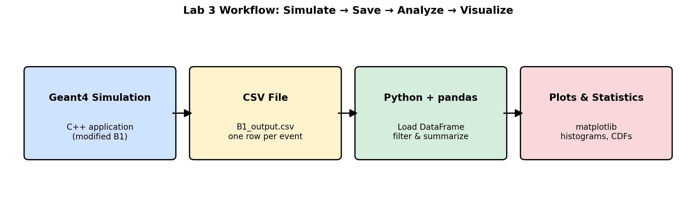
Once we have the data, we will switch hats from a simulation user to a data analyst. We will use the powerful Python programming language along with two essential libraries: pandas for data manipulation and matplotlib for plotting. You will write a script to read the CSV file and generate a histogram, which is a graph that shows the frequency distribution of the energy deposition values. This process—simulate, save, analyze, visualize—is a fundamental cycle in computational science.

Prerequisites

Before you begin, ensure you have the following:

Completed Lab 2 (successfully built and ran Example B1)
Text editor for C++ code (gedit, nano, or VS Code)
Basic understanding of C++ syntax (we’ll guide you through the modifications)
Python 3 installed (should be pre-installed on Ubuntu)

Pre-Lab Questions

What is a CSV file? Why is it a good choice for this lab compared to a more complex format like ROOT?
What is a histogram and what does it show?
Briefly describe the roles of the pandas and matplotlib Python libraries.
In Geant4, what is the difference between a “Run”, an “Event”, and a “Step”?
What does it mean to “score” a quantity in a simulation?

Step 1: Set Up the Lab and Review the Code Structure

Create a new directory for this lab and copy the B1 example into it, just as you did in Lab 2:

mkdir -p ~/g4-labs/lab3
cd ~/g4-labs/lab3
cp -r ~/geant4-v11.3.2/examples/basic/B1 .
cd B1

Before we start modifying, let’s understand the key files and the Geant4 action hierarchy:

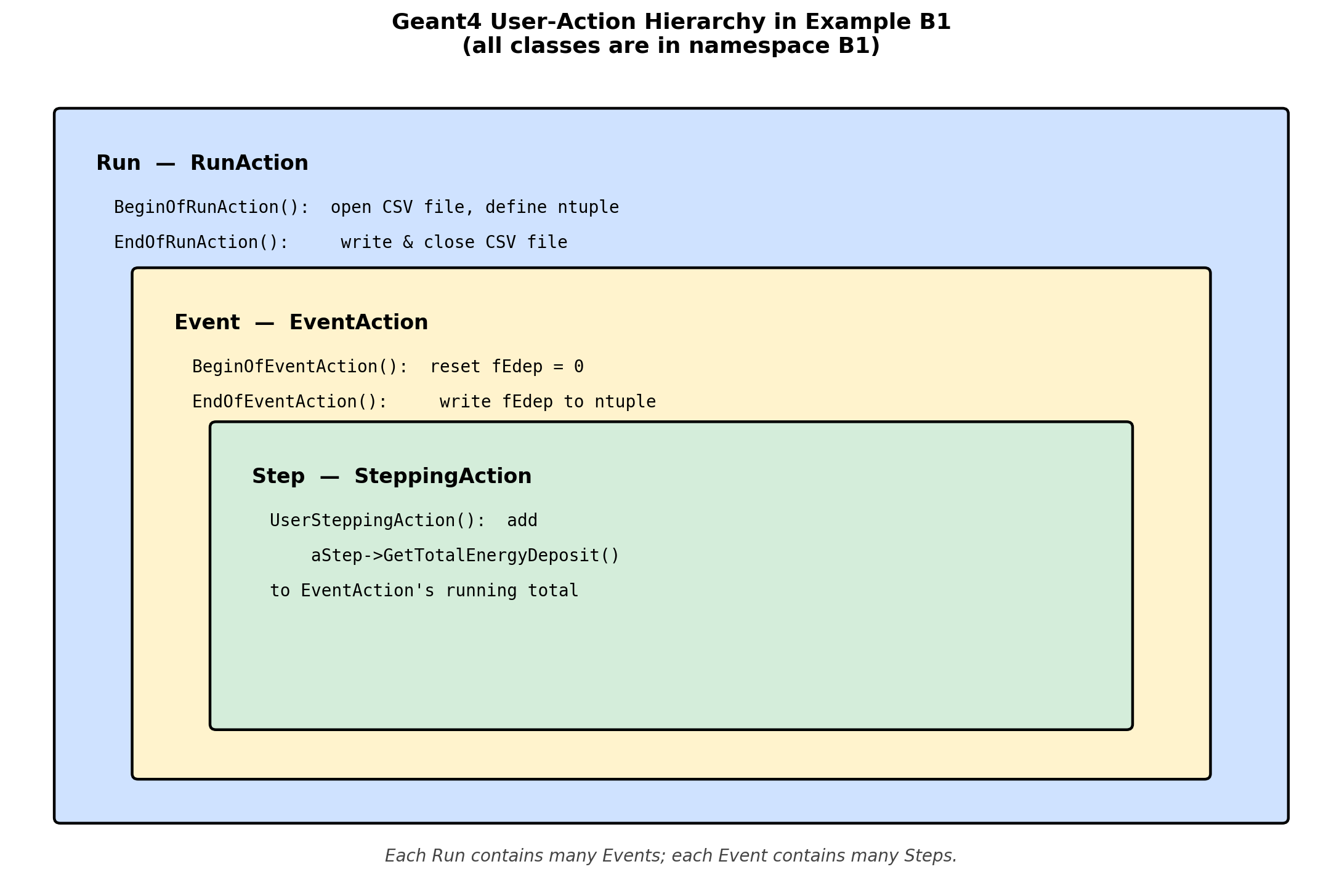
Geant4 User Action Classes

In the modern B1 example, all of these classes live inside namespace B1 { ... }. The header and source files do not carry a B1 filename prefix — for example, the run-action class is declared as class RunAction inside namespace B1, in include/RunAction.hh. Every code addition you make in this lab will go inside an existing namespace B1 block in the corresponding .cc file.

Familiarize yourself with these key files:
- include/RunAction.hh & src/RunAction.cc:
  - Controls actions at the beginning and end of a Run (a collection of events)
  - We will edit the source file to open, write, and close the CSV output
- include/EventAction.hh & src/EventAction.cc:
  - Controls actions at the beginning and end of each Event (simulation of one primary particle)
  - We will edit the source file to record one row of CSV data per event
- src/SteppingAction.cc:
  - Executed at every single Step a particle takes through the geometry
  - The example already collects per-step energy here. We will not modify this file.
Open src/SteppingAction.cc in a text editor and read through UserSteppingAction:
```
gedit src/SteppingAction.cc &
```
Notice that the example already extracts each step’s energy deposit and adds it to the event total via fEventAction->AddEdep(edepStep). The data lives in memory but never reaches disk — fixing that is what this lab is about.

Step 2: Modify C++ Code to Save Data

What the example already does

Before we add anything, look at how energy already flows through the unmodified B1 example. Open these three files in your editor and find the lines below — you do not need to change them:

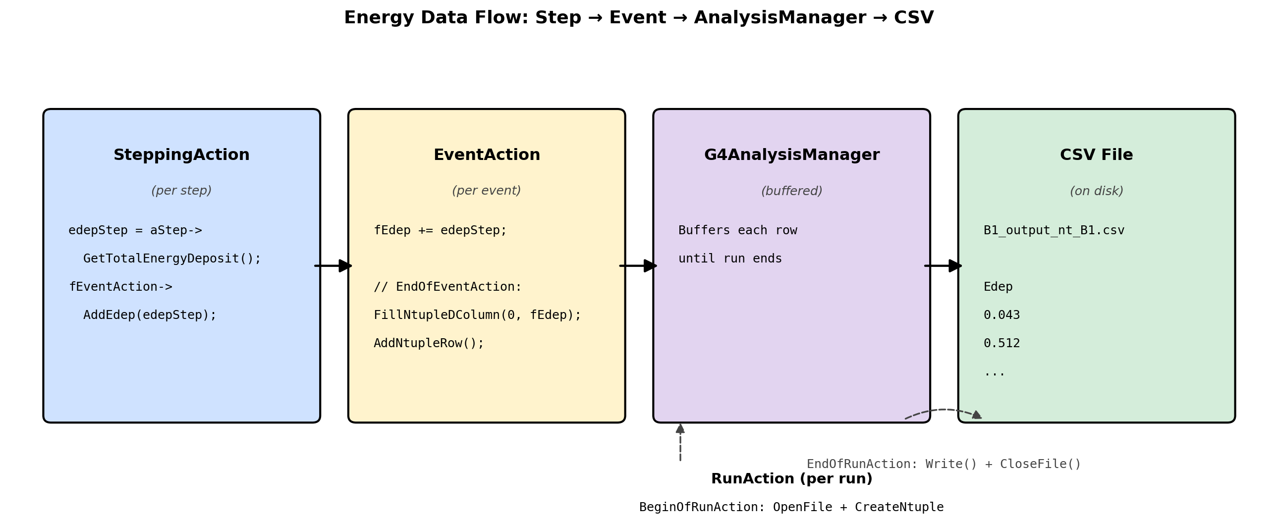
include/EventAction.hh already declares the helper and the per-event accumulator:
```
void AddEdep(G4double edep) { fEdep += edep; }
G4double fEdep = 0.;
```

src/EventAction.cc already resets fEdep at the start of each event and forwards it to the run action at the end:

void EventAction::BeginOfEventAction(const G4Event*)  { fEdep = 0.; }
void EventAction::EndOfEventAction(const G4Event*)   { fRunAction->AddEdep(fEdep); }

src/SteppingAction.cc already accumulates each step’s deposit into the event total:

G4double edepStep = step->GetTotalEnergyDeposit();
fEventAction->AddEdep(edepStep);

So the per-step → per-event → per-run pipeline is already wired up. The energy lands in fEdep at the end of each event. Our only job in this lab is to also write that value to a CSV file.

What we’ll change

There are exactly two files to edit:

src/RunAction.cc — set up the CSV file at the start of the run and write/close it at the end.
src/EventAction.cc — at the end of each event, write fEdep as one new row of the CSV.

That’s it. Two #include additions and ~12 new lines of code in total.

Modification 1: RunAction.cc

We use G4AnalysisManager, Geant4’s built-in writer that supports CSV, ROOT, XML, and HDF5. We’ll use CSV.

Open src/RunAction.cc:
```
gedit src/RunAction.cc &
```
Add the analysis-manager header near the other #include lines at the top:
```
#include "G4AnalysisManager.hh"
```

Inside RunAction::BeginOfRunAction(const G4Run*), add the following block (anywhere inside the function body is fine — putting it at the top is conventional):

// --- Lab 3 addition: open CSV and define the per-event ntuple ---
auto analysisManager = G4AnalysisManager::Instance();
analysisManager->SetDefaultFileType("csv");
analysisManager->OpenFile("B1_output");

analysisManager->CreateNtuple("B1", "Energy Deposition Data");
analysisManager->CreateNtupleDColumn("Edep");  // column 0
analysisManager->FinishNtuple();

What this does: Tells the analysis manager to write CSV, gives the file a name (B1_output), and declares one ntuple column called Edep. Each row will hold one event’s fEdep.

Inside RunAction::EndOfRunAction(const G4Run* run), add the following at the very end of the function (after the existing G4cout print block):

// --- Lab 3 addition: flush and close the CSV ---
auto analysisManager = G4AnalysisManager::Instance();
analysisManager->Write();
analysisManager->CloseFile();

Modification 2: EventAction.cc

Open src/EventAction.cc:
```
gedit src/EventAction.cc &
```
Add the analysis-manager header near the top:
```
#include "G4AnalysisManager.hh"
```

Find the existing EventAction::EndOfEventAction function. It currently looks like this — do not retype it, you are only locating it:

void EventAction::EndOfEventAction(const G4Event*)
{
  // accumulate statistics in run action
  fRunAction->AddEdep(fEdep);
}

Inside that function, after the existing fRunAction->AddEdep(fEdep); line and before the closing }, paste these four lines (and only these four lines):

// --- Lab 3 addition: also write fEdep to the CSV ---
auto analysisManager = G4AnalysisManager::Instance();
analysisManager->FillNtupleDColumn(0, fEdep);
analysisManager->AddNtupleRow();

After your edit, the complete function should read:

void EventAction::EndOfEventAction(const G4Event*)
{
  // accumulate statistics in run action
  fRunAction->AddEdep(fEdep);

  // --- Lab 3 addition: also write fEdep to the CSV ---
  auto analysisManager = G4AnalysisManager::Instance();
  analysisManager->FillNtupleDColumn(0, fEdep);
  analysisManager->AddNtupleRow();
}

What this does: Each event ends with one new row in the CSV containing the total energy deposited in the scoring volume during that event.

Summary of Modifications

You’ve now modified two files:

File	Change
`src/RunAction.cc`	Add `G4AnalysisManager.hh`; open the CSV in `BeginOfRunAction`, write/close it in `EndOfRunAction`
`src/EventAction.cc`	Add `G4AnalysisManager.hh`; in `EndOfEventAction`, fill one ntuple row per event

Note that EventAction.hh, SteppingAction.cc, and the energy-accumulation logic itself were left untouched — the example already had everything we needed up to the point of writing to disk.

Step 3: Compile and Run the Modified Application

Now let’s compile your modified code and generate some data!

Navigate to the build directory (create one if it doesn’t exist):
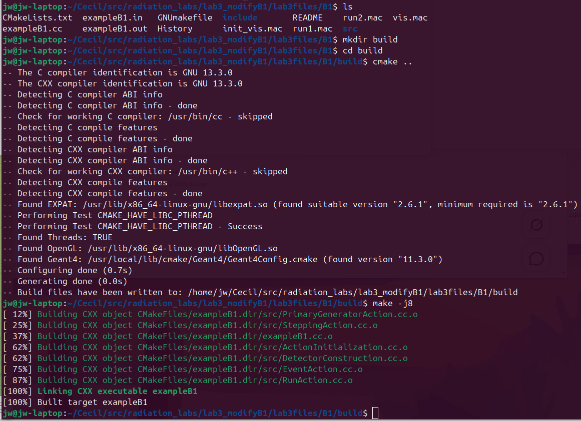
```
mkdir -p build
cd build
```
Configure the build with CMake:
```
cmake ..
```
Compile the modified application:
```
make -j$(nproc)
```
If you encounter errors, carefully check your code modifications against the instructions. Common issues:
- Missing semicolons
- Incorrect placement of code
- Typos in variable names

Create a macro file for data collection. In the B1 directory (not build), create lab3.mac:

cd ..
nano lab3.mac

Add these contents:

# Lab 3 Data Collection Run
# Simulate 10,000 events with default 6 MeV gammas

# Force single-threaded mode so we get ONE CSV file, not one per worker.
# Must come BEFORE /run/initialize.
/run/numberOfThreads 1

/run/initialize
/run/printProgress 1000
/run/beamOn 10000

This will run 10,000 events and print progress every 1,000 events. /run/numberOfThreads 1 keeps Geant4 from running multi-threaded, which would otherwise produce one CSV file per worker thread.

Run the simulation:
```
cd build
./exampleB1 ../lab3.mac
```
After completion, list the CSV files:
```
ls -lh *.csv
```
You should see one file named B1_output_nt_B1_t0.csv. Geant4’s CSV writer always appends a _tN worker-thread suffix; with one thread, that’s _t0. If you see multiple _tN.csv files, you forgot /run/numberOfThreads 1 — delete them and re-run.
View the first few lines:
```
head -20 B1_output_nt_B1_t0.csv
```
You should see a header row followed by numerical energy values in MeV.

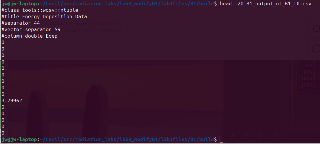
Step 4: Install Python Analysis Libraries

Before we can analyze our data, we need to install the required Python packages.

First, check if pip is installed:
```
pip3 --version
```
If needed, install pip:
```
sudo apt install python3-pip
```
Install pandas and matplotlib:
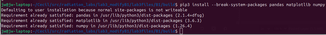
```
pip3 install --break-system-packages pandas matplotlib numpy
```
Why the --break-system-packages flag? Recent versions of Ubuntu (24.04+) follow PEP 668 and mark the system Python environment as “externally managed”, so a plain pip3 install pandas will refuse to run with an error: externally-managed-environment message. The flag tells pip to install into the user site-packages directory anyway, which is fine for this VM-based course where we are not maintaining the host system. (In a production environment you would create a virtual environment with python3 -m venv instead.)

These packages provide:
- pandas: Data manipulation and analysis
- matplotlib: Creating visualizations and plots
- numpy: Numerical computing (dependency for pandas)

Verify the installation:

python3 -c "import pandas; import matplotlib; print('Success!')"

Step 5: Analyze the Data with Python - Basic Analysis

Now let’s create a Python script to analyze our simulation data.

In your B1/build directory, create analyze_basic.py:

nano analyze_basic.py

Paste the following content. Important: the code must start at column 0 (no leading whitespace), or Python will reject it with IndentationError: unexpected indent.

import pandas as pd
import matplotlib.pyplot as plt

# --- Load the Data ---
# Geant4's CSV output begins with metadata lines starting with '#'
# (e.g. "#class tools::wcsv::ntuple", "#column double Edep").
# We tell pandas to skip those and supply the column name ourselves.
print("=" * 50)
print("GEANT4 SIMULATION DATA ANALYSIS")
print("=" * 50)
print("\nReading data from B1_output_nt_B1_t0.csv...")

data = pd.read_csv('B1_output_nt_B1_t0.csv',
                   comment='#', header=None, names=['Edep'])

print(f"Data loaded: {len(data)} events, shape {data.shape}")
print("\nFirst 10 energy deposition values (MeV):")
print(data.head(10))

# --- Basic Statistics ---
print("\n" + "=" * 50)
print("BASIC STATISTICS")
print("=" * 50)

mean_edep = data['Edep'].mean()
std_edep = data['Edep'].std()
median_edep = data['Edep'].median()

print(f"Mean Energy Deposition:     {mean_edep:.4f} MeV")
print(f"Standard Deviation:         {std_edep:.4f} MeV")
print(f"Median:                     {median_edep:.4f} MeV")
print(f"Minimum:                    {data['Edep'].min():.4f} MeV")
print(f"Maximum:                    {data['Edep'].max():.4f} MeV")

percentiles = data['Edep'].quantile([0.25, 0.5, 0.75, 0.90, 0.95])
print(f"\nPercentiles:")
print(f"  25th percentile (Q1):     {percentiles[0.25]:.4f} MeV")
print(f"  50th percentile (median): {percentiles[0.50]:.4f} MeV")
print(f"  75th percentile (Q3):     {percentiles[0.75]:.4f} MeV")
print(f"  90th percentile:          {percentiles[0.90]:.4f} MeV")
print(f"  95th percentile:          {percentiles[0.95]:.4f} MeV")

# --- Histogram ---
plt.figure(figsize=(12, 8))
plt.hist(data['Edep'], bins=100, alpha=0.75,
         color='steelblue', edgecolor='black')
plt.axvline(mean_edep, color='red', linestyle='--',
            linewidth=2, label=f'Mean: {mean_edep:.3f} MeV')
plt.axvline(median_edep, color='green', linestyle='--',
            linewidth=2, label=f'Median: {median_edep:.3f} MeV')

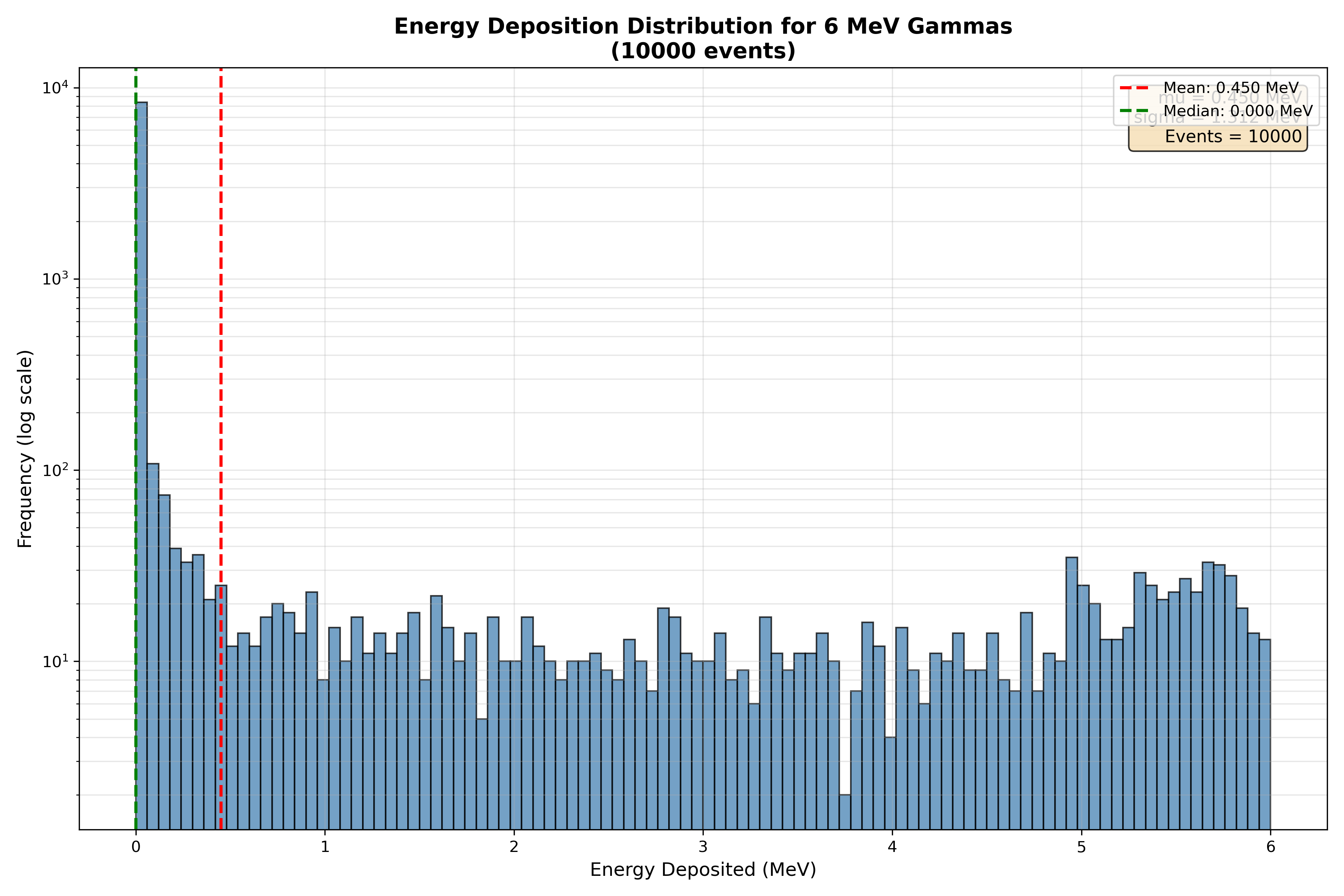
plt.title(f'Energy Deposition Distribution for 6 MeV Gammas\n({len(data)} events)',
          fontsize=14, fontweight='bold')
plt.xlabel('Energy Deposited (MeV)', fontsize=12)
plt.ylabel('Frequency (log scale)', fontsize=12)
plt.yscale('log')
plt.grid(True, alpha=0.3, which='both')
plt.legend(fontsize=10)

stats_text = f'mu = {mean_edep:.3f} MeV\nsigma = {std_edep:.3f} MeV\nEvents = {len(data)}'
plt.text(0.98, 0.97, stats_text, transform=plt.gca().transAxes,
         fontsize=11, verticalalignment='top', horizontalalignment='right',
         bbox=dict(boxstyle='round', facecolor='wheat', alpha=0.8))

plt.tight_layout()
plt.savefig('edep_histogram.png', dpi=300)
print("\nHistogram saved to edep_histogram.png")

Save and close, then run:

python3 analyze_basic.py

View the generated histogram:

eog edep_histogram.png

(Or use your preferred image viewer.)

Step 6: Advanced Analysis - Data Filtering and Comparison

Let’s explore pandas’ powerful data manipulation capabilities by filtering the data and creating comparative visualizations.

Create analyze_advanced.py:

nano analyze_advanced.py

Paste the following content (must start at column 0 — no leading whitespace):

import pandas as pd
import matplotlib.pyplot as plt
import numpy as np

print("Loading simulation data...")
data = pd.read_csv('B1_output_nt_B1_t0.csv',
                   comment='#', header=None, names=['Edep'])

# --- Data Filtering Examples ---
print("\n" + "=" * 50)
print("DATA FILTERING EXAMPLES")
print("=" * 50)

high_energy = data[data['Edep'] > 4.0]
print(f"\nEvents with Edep > 4.0 MeV: {len(high_energy)} "
      f"({len(high_energy)/len(data)*100:.1f}%)")

low_energy = data[data['Edep'] < 1.0]
print(f"Events with Edep < 1.0 MeV: {len(low_energy)} "
      f"({len(low_energy)/len(data)*100:.1f}%)")

zero_energy = data[data['Edep'] == 0.0]
print(f"Events with Edep = 0.0 MeV: {len(zero_energy)} "
      f"({len(zero_energy)/len(data)*100:.1f}%)")
print("  -> These are events where the particle passed through "
      "without interacting")

mid_range = data[(data['Edep'] >= 2.0) & (data['Edep'] <= 4.0)]
print(f"Events with 2.0 <= Edep <= 4.0 MeV: {len(mid_range)} "
      f"({len(mid_range)/len(data)*100:.1f}%)")

# --- Multi-Panel Figure ---
fig, axes = plt.subplots(2, 2, figsize=(14, 10))
fig.suptitle('Advanced Energy Deposition Analysis',
             fontsize=16, fontweight='bold')

# Panel 1: Full distribution (log y to see the tail past the zero spike)
ax1 = axes[0, 0]
ax1.hist(data['Edep'], bins=100, color='steelblue',
         alpha=0.7, edgecolor='black')
ax1.set_xlabel('Energy Deposited (MeV)')
ax1.set_ylabel('Frequency (log scale)')
ax1.set_yscale('log')
ax1.set_title(f'Full Distribution (n={len(data)})')
ax1.grid(True, alpha=0.3, which='both')

# Panel 2: Excluding zero-energy events (log y for the long tail)
ax2 = axes[0, 1]
non_zero = data[data['Edep'] > 0]
ax2.hist(non_zero['Edep'], bins=80, color='coral',
         alpha=0.7, edgecolor='black')
ax2.set_xlabel('Energy Deposited (MeV)')
ax2.set_ylabel('Frequency (log scale)')
ax2.set_yscale('log')
ax2.set_title(f'Non-Zero Events Only (n={len(non_zero)})')
ax2.grid(True, alpha=0.3, which='both')

# Panel 3: Cumulative distribution
ax3 = axes[1, 0]
sorted_data = np.sort(data['Edep'])
cumulative = np.arange(1, len(sorted_data) + 1) / len(sorted_data) * 100
ax3.plot(sorted_data, cumulative, linewidth=2, color='darkgreen')
ax3.set_xlabel('Energy Deposited (MeV)')
ax3.set_ylabel('Cumulative Percentage (%)')
ax3.set_title('Cumulative Distribution Function')
ax3.grid(True, alpha=0.3)
ax3.axhline(50, color='red', linestyle='--', alpha=0.5, label='50%')
ax3.axhline(95, color='orange', linestyle='--', alpha=0.5, label='95%')
ax3.legend()

# Panel 4: Box plot
ax4 = axes[1, 1]
box_data = [data['Edep'], non_zero['Edep']]
bp = ax4.boxplot(box_data, labels=['All Events', 'Non-Zero Only'],
                 patch_artist=True, showmeans=True)
for patch, color in zip(bp['boxes'], ['lightblue', 'lightcoral']):
    patch.set_facecolor(color)
ax4.set_ylabel('Energy Deposited (MeV)')
ax4.set_title('Box Plot Comparison')
ax4.grid(True, alpha=0.3, axis='y')

plt.tight_layout()
plt.savefig('edep_advanced_analysis.png', dpi=300)
print("\nAdvanced analysis figure saved to edep_advanced_analysis.png")

# --- Statistical Comparison ---
print("\n" + "=" * 50)
print("STATISTICAL COMPARISON")
print("=" * 50)
print("\nAll Events:")
print(f"  Mean:   {data['Edep'].mean():.4f} MeV")
print(f"  Median: {data['Edep'].median():.4f} MeV")
print(f"  Std:    {data['Edep'].std():.4f} MeV")
print("\nNon-Zero Events Only:")
print(f"  Mean:   {non_zero['Edep'].mean():.4f} MeV")
print(f"  Median: {non_zero['Edep'].median():.4f} MeV")
print(f"  Std:    {non_zero['Edep'].std():.4f} MeV")

print("\n" + "=" * 50)
print("DETAILED SUMMARY STATISTICS")
print("=" * 50)
print(data['Edep'].describe())

Run it and view the figure:

python3 analyze_advanced.py
eog edep_advanced_analysis.png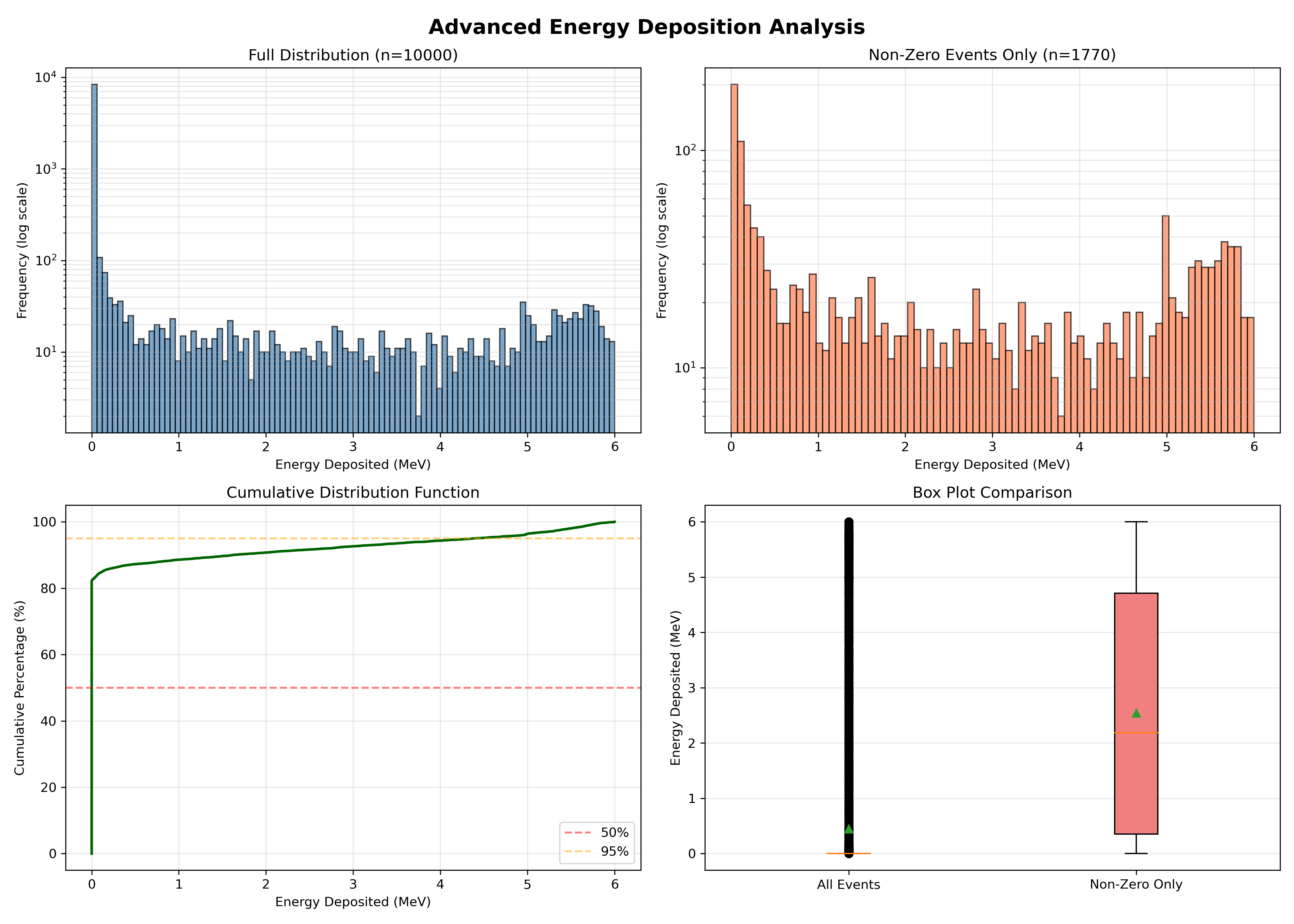

Step 7: Comparing Different Particle Types

Let’s generate data for different particles and compare their energy deposition patterns.

Create macro files for different particles. First, protons:

cd ~/g4-labs/lab3/B1
nano proton_beam.mac

Add:

/run/numberOfThreads 1
/run/initialize
/gun/particle proton
/gun/energy 150 MeV
/run/printProgress 1000
/run/beamOn 10000

Create electron beam macro:

nano electron_beam.mac

Add:

/run/numberOfThreads 1
/run/initialize
/gun/particle e-
/gun/energy 50 MeV
/run/printProgress 1000
/run/beamOn 10000

Run simulations and rename output files. Remember: each run produces B1_output_nt_B1_t0.csv, so we rename it after each run before it gets overwritten.

cd build

# Run gamma simulation (already done, but let's be explicit)
./exampleB1 ../lab3.mac
mv B1_output_nt_B1_t0.csv gamma_6MeV.csv

# Run proton simulation
./exampleB1 ../proton_beam.mac
mv B1_output_nt_B1_t0.csv proton_150MeV.csv

# Run electron simulation
./exampleB1 ../electron_beam.mac
mv B1_output_nt_B1_t0.csv electron_50MeV.csv

Create the comparison script:

nano compare_particles.py

Paste the following content (must start at column 0 — no leading whitespace):

import pandas as pd
import matplotlib.pyplot as plt

# All three CSVs were produced by the modified B1, so they share the
# same Geant4 header format. We supply the column name ourselves.
read_kwargs = dict(comment='#', header=None, names=['Edep'])

print("Loading particle data...")
gamma_data    = pd.read_csv('gamma_6MeV.csv',    **read_kwargs)
proton_data   = pd.read_csv('proton_150MeV.csv', **read_kwargs)
electron_data = pd.read_csv('electron_50MeV.csv', **read_kwargs)

fig, axes = plt.subplots(2, 2, figsize=(14, 10))
fig.suptitle('Particle Type Comparison: Energy Deposition',
             fontsize=16, fontweight='bold')

ax1 = axes[0, 0]
ax1.hist(gamma_data['Edep'], bins=80, alpha=0.7,
         color='blue', label='6 MeV gamma', edgecolor='black')
ax1.set_xlabel('Energy Deposited (MeV)')
ax1.set_ylabel('Frequency (log scale)')
ax1.set_yscale('log')
ax1.set_title('Gamma Rays (6 MeV)')
ax1.legend()
ax1.grid(True, alpha=0.3, which='both')

ax2 = axes[0, 1]
ax2.hist(proton_data['Edep'], bins=80, alpha=0.7,
         color='red', label='150 MeV p+', edgecolor='black')
ax2.set_xlabel('Energy Deposited (MeV)')
ax2.set_ylabel('Frequency (log scale)')
ax2.set_yscale('log')
ax2.set_title('Protons (150 MeV)')
ax2.legend()
ax2.grid(True, alpha=0.3, which='both')

ax3 = axes[1, 0]
ax3.hist(electron_data['Edep'], bins=80, alpha=0.7,
         color='green', label='50 MeV e-', edgecolor='black')
ax3.set_xlabel('Energy Deposited (MeV)')
ax3.set_ylabel('Frequency (log scale)')
ax3.set_yscale('log')
ax3.set_title('Electrons (50 MeV)')
ax3.legend()
ax3.grid(True, alpha=0.3, which='both')

# Normalized overlay (log y so the three shapes are comparable across orders)
ax4 = axes[1, 1]
ax4.hist(gamma_data['Edep'], bins=60, alpha=0.5, color='blue',
         label=f'gamma (mu={gamma_data["Edep"].mean():.2f})', density=True)
ax4.hist(proton_data['Edep'], bins=60, alpha=0.5, color='red',
         label=f'p+ (mu={proton_data["Edep"].mean():.2f})', density=True)
ax4.hist(electron_data['Edep'], bins=60, alpha=0.5, color='green',
         label=f'e- (mu={electron_data["Edep"].mean():.2f})', density=True)
ax4.set_xlabel('Energy Deposited (MeV)')
ax4.set_ylabel('Probability Density (log scale)')
ax4.set_yscale('log')
ax4.set_title('Normalized Overlay Comparison')
ax4.legend()
ax4.grid(True, alpha=0.3, which='both')

plt.tight_layout()
plt.savefig('particle_comparison.png', dpi=300)
print("Comparison figure saved to particle_comparison.png")

print("\n" + "=" * 60)
print("STATISTICAL COMPARISON BY PARTICLE TYPE")
print("=" * 60)

for name, df in [('Gamma (6 MeV)',    gamma_data),
                 ('Proton (150 MeV)', proton_data),
                 ('Electron (50 MeV)', electron_data)]:
    n_zero = (df['Edep'] == 0).sum()
    print(f"\n{name}:")
    print(f"  Mean:        {df['Edep'].mean():.4f} MeV")
    print(f"  Median:      {df['Edep'].median():.4f} MeV")
    print(f"  Std Dev:     {df['Edep'].std():.4f} MeV")
    print(f"  Max:         {df['Edep'].max():.4f} MeV")
    print(f"  Zero events: {n_zero} ({n_zero/len(df)*100:.1f}%)")

Run it:

python3 compare_particles.py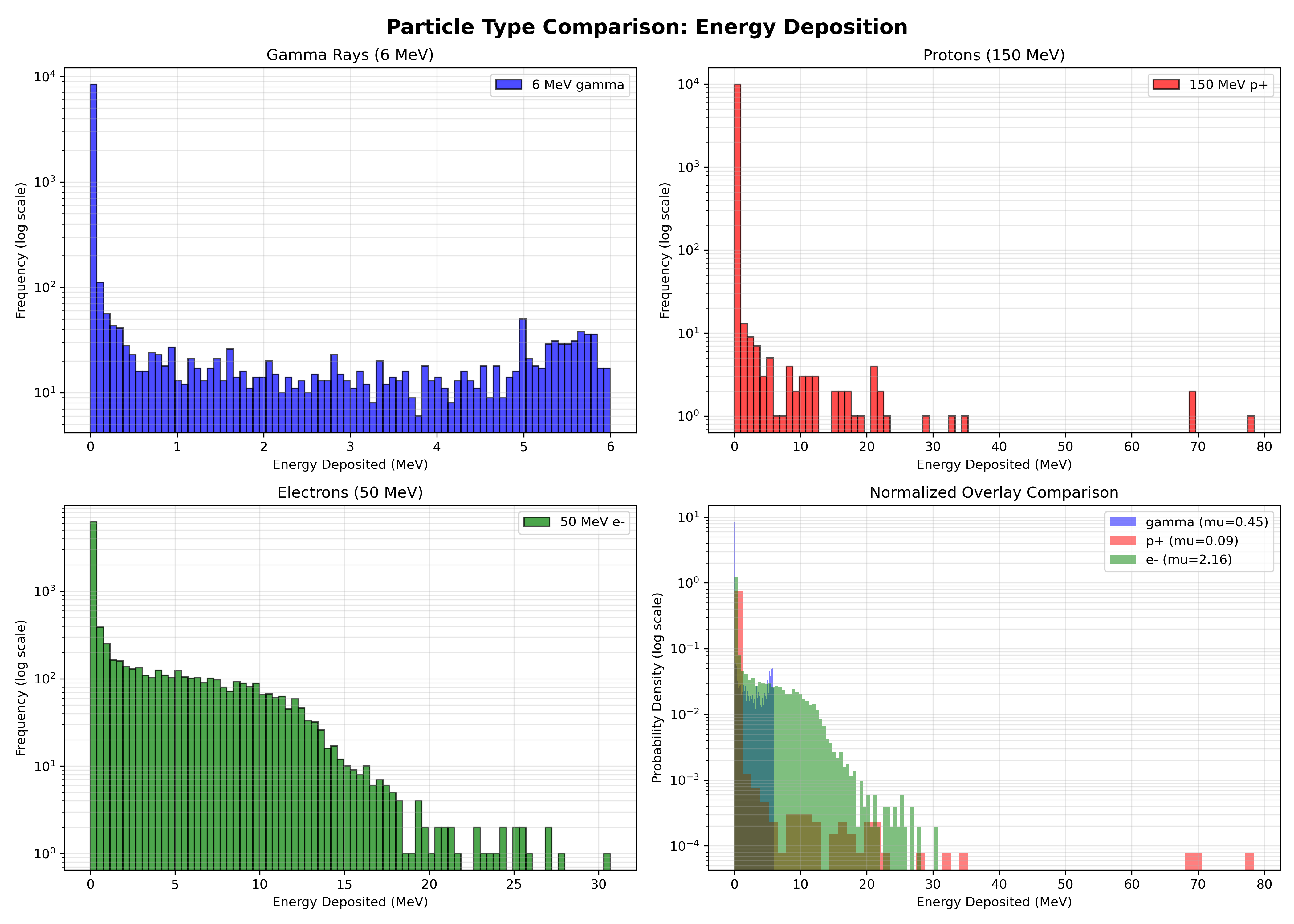

Analysis Questions

Now that you have generated and analyzed the data, answer these questions:

Part 1: Understanding the Distribution

Describe the shape of the energy deposition histogram for gamma rays. Is the energy deposition the same for every event?
Why is there a distribution of values instead of a single value? Consider:
- Stochastic nature of particle interactions
- Different interaction mechanisms (photoelectric, Compton, pair production)
- Variation in secondary particle production
The peak of the distribution represents the most probable energy deposition. What is this value approximately? How does it compare to the initial energy of the gamma particle (6 MeV)?
Explain why the deposited energy is typically lower than the incident energy. (Hint: Does the particle always deposit all of its energy in the detector?)

Part 2: Understanding Zero Energy Events

What percentage of events have zero energy deposition? What does this represent physically?
Why would a 6 MeV gamma ray pass through the detector without depositing any energy?

Part 3: Comparing Particle Types

Compare the mean energy deposition for:
- 6 MeV gammas
- 150 MeV protons
- 50 MeV electrons
Which particle type deposits the most energy on average? Why?
Which particle type has the most consistent energy deposition (smallest standard deviation)? Explain this in terms of the physics of how each particle type interacts with matter.
Notice the shape differences in the distributions:
- Gammas: Broad, exponential-like distribution
- Protons: Sharp, peaked distribution
- Electrons: Intermediate characteristics
Explain these shape differences based on the interaction mechanisms of each particle type.

Part 4: Pandas Data Analysis

In the advanced analysis script, we filtered events with data[data['Edep'] > 4.0]. Explain in plain English what this pandas operation does.
What is the advantage of using pandas DataFrames versus manipulating the CSV file directly with basic Python?
The cumulative distribution plot shows what percentage of events have energy deposition below a certain value. What is the energy value at which 50% of events fall below? What is this called statistically?

Part 5: Scientific Workflow

Why is CSV a good intermediate format for this analysis workflow (Geant4 → CSV → Python)?
How would you modify the code to save additional information, such as:
- The number of steps per event
- Energy deposited in different detector volumes
- Particle type information for secondary particles

Troubleshooting

Common issues and solutions:

“No module named ‘pandas’”: Install with pip3 install --break-system-packages pandas matplotlib numpy.
error: externally-managed-environment from pip: Ubuntu 24.04+ marks the system Python as managed (PEP 668). Re-run with --break-system-packages, as shown in Step 4.
Many B1_output_nt_B1_tN.csv files instead of one _t0.csv: Geant4 ran multi-threaded and each worker thread wrote its own CSV. Add /run/numberOfThreads 1 to your macro before /run/initialize, delete the per-thread files (rm B1_output_nt_B1_t*.csv), and re-run.
CSV file not found: Make sure you’re running Python from the build directory and that the filename in pd.read_csv(...) matches what ls *.csv shows.
Empty histogram: Check that your CSV file has data and proper column headers
Compilation errors: Verify all code modifications carefully match the instructions
G4AnalysisManager errors: Ensure you’ve included the header file in all necessary source files

Conclusion

You have successfully modified a Geant4 application to output data, run simulations with different particle types, and performed sophisticated data analysis using Python’s pandas and matplotlib libraries. You’ve learned:

How Geant4’s action classes work together to record simulation data
The modern approach to data output using G4AnalysisManager
Essential pandas operations for data manipulation and analysis
Creating publication-quality visualizations with matplotlib
The scientific workflow from simulation to analysis to visualization

These skills are fundamental for computational physics and will be used throughout the remainder of this course and in professional scientific computing work.

References

Geant4 Collaboration. (n.d.). Geant4 Analysis Tools Documentation
Hrivnacova, I. (2018). Using Geant4 Analysis Manager
Hrivnacova, I. (2023). Geant4 Analysis Tools Tutorial
McKinney, W. (2010). Data Structures for Statistical Computing in Python
Hunter, J. D. (2007). Matplotlib: A 2D Graphics Environment
The Python Graph Gallery. (n.d.). Histogram Examples

Additional Resources

Optional Extensions

If you finish early or want to explore further:

Add More Columns: Modify the code to save additional data:
- Track length
- Number of steps
- Particle position at end of event
Different Geometries: Modify the detector geometry in DetectorConstruction.cc and observe how it affects energy deposition
Energy Scan: Create a script that runs simulations at multiple energies (e.g., 1, 2, 4, 6, 8, 10 MeV) and plots how mean energy deposition varies with incident energy
Interactive Plotting: Modify the Python scripts to use plt.show() for interactive exploration of the data
Statistical Tests: Use scipy to perform statistical tests comparing different datasets (t-tests, KS tests, etc.)